DSC80 Note (Simplified Version)
This is the summary note of DSC80(Fall 2019) in UCSD. Part of this note is derived from the course jupyter notebook. This is the link of this course’s main page: https://sites.google.com/eng.ucsd.edu/dsc-80-fall-2019
Notes
Lecture 1 & 2
axis = 0 和 axis = 1的区别记忆:
一般方法的默认都是axis=0
然后axis = 1就是方法结束后行数是不会变的, axis = 0方法结束之后列数是不会变的
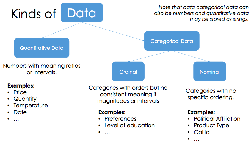
Lecture 3. Messay data
-
quantiattive data math model on it
-
Categorical data
- Ordinal: can’t do math
- Nominal: just labels, no order
# Danger! 就是强行的数据类型的转换,然后有error的地方就设置为NaN
df['DSC 80 Final Grade'] = pd.to_numeric(df['DSC 80 Final Grade'], errors='coerce')
- The result of any comparison (=,!=,<,>) with
NaNisFalse.- Use functions for checking null:
np.isnan,np.isnull
- Use functions for checking null:
-
NaNis of float-type. - Be careful of Pandas type-coercian with
NaN!
Lecture 4. Testing Hypotheses
1. test statistic
Measure information that answers the questions we’re trying to answer.
- Difference in means: is similar to the absolute difference in means except that the difference is “directional”. When you use the difference in means as a test statistic in a permutation test, you must specify the direction of your alternative hypothesis.
- Absolute difference in means: compares a measure of center of the two distributions
- KS: compares the overall shape of the two distributions. Have lower p-values. In cases where you want to test whether two quantitative distributions are different, the ks statistic is often more preferable for this reason.
2. Null and alternative
- The method only works if we can simulate data under one of the hypotheses.
- Null hypothesis:
Often (but not always) the null hypothesis states there is no association or difference between variables or subpopulations. Null hyp必然是俩sample相等,也就是A = B这样的.- A well defined probability model about how the data were generated
- We can simulate data under the assumptions of this model – “under the null hypothesis”
- Alternative hypothesis:
Hypothesis that sample observations are influenced by some non-random cause (unlike Null Hypothesis). Altern hyp必然是俩sample不等的样子,至于是> / < / !=, 取决于你想要test什么.如果你想要测试A > B,那altern hy就是A > B.- A different view about the origin of the data
3. P-value (observed significance level)
The P-value is the chance, under the null hypothesis, that the test statistic is equal to the value that was observed in the data or is even further in the direction of the alternative.
-
“Inconsistent”: The test statistic is in the tail of the empirical distribution under the null hypothesis
- “In the tail,” first convention:
- The area in the tail is less than 5%
- The result is “statistically significant”
- “In the tail,” second convention:
- The area in the tail is less than 1%
- The result is “highly statistically significant”
Lecture 5. Data Granularity
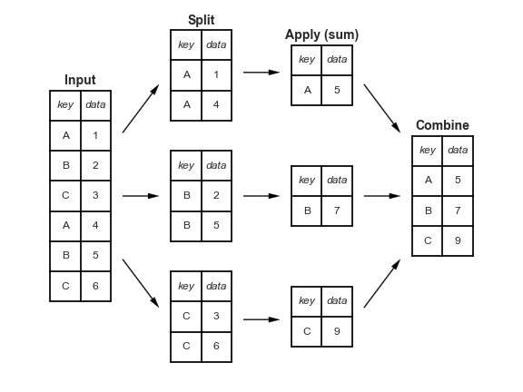
- split breaks up and groups a
DataFramedepending on the value of the specified key. - apply computes a function (e.g. aggregate, transformation, or filtering) within the individual groups.
- combine merges the results of these operations into an output array.
-
dataframe.groupby(key)returns aDataFrameGroupByobject. -
.groupis a dictionary of grouping keys and the corresponding dataframe -
.get_group(key)method returns a dataframe corresponding to the given key
- We will commonly combine
groupbywith column selection:- e.g.,
df.groupby("Region")["Sales"]
- e.g.,
- Then add an aggregate calculation on that column:
aggregate:
# aggregate

def avg_str_len(series):
    return series.str.len().mean()  # purpose?

res = (
    people
        .groupby(["Color", "Gender"])
        .aggregate({"Name": avg_str_len, "Number": np.mean})  #就是把方法用到那个列上面
)
pivot / pivot_table
Lecture 6. combining data
1. pd.concat()
上下合并 pd.concat([class_1,class_2], ignore_index=True)
2. merge()
df3 = df1.merge(df2) 默认采用inner merge
merge的方法选择使用how属性: df3_outer = pd.merge(df1, df2, how = "outer") 总共4种:
- inner
- outer
- left
- right
若俩df有好几个相同的列,那么要用on来表示根据哪一列来merge
可以加suffix = ()来区分那些没选中的相同列
3. join()
df1.join(df2) 默认采用left join
是根据df2的索引来join的
Lecture 7. permutation test
1. Testing through simulation
- Statistic: Difference between means.
- Null hypothesis: The two groups are sampled from the same distribution.
- Note that the null hypothesis doesn’t say what the distribution is.我感觉这就是判断用hyp还是per的关键处,就是simul的时候,能不能直接根据distr来生成samples
- Different from jury panel example, fair coin example, etc.
- We can’t draw directly from the distribution!
- We have to do something a bit more clever.
2. Permutation tests
- Perhaps the difference in means we saw is due to random chance in assignment.
- Permutation test: Shuffle the group labels a bunch of times; how often do we see a statistic this extreme?
- Randomly permuting labels is equivalent to randomly assigning birth weights to groups (without changing group sizes)
- If we rarely see something this extreme, then the null hypothesis doesn’t look likely.
It doesn’t matter which column we shuffle!
3. Permutation Test Summary
- A permutation test is a hypothesis test
- Null hypothesis states “two observations come from same distribution”. (空假设就是俩分布相等)
- Simulate null hypothesis using permutations.
- Don’t have to know what the distributions are!
- When test-statistic is is difference-in-means <=> two sample t-test
- Permutation tests are more generally applicable.
4. Permutation使用总结
凡是使用到permutation其实就是会出现俩variables.
- 一个var必然是categorical的,就是按照这个来归类的(设该var为G).
- 另外一个var有两种情况:
- 一种是这个var是quantitative的,这样就直接使用groupby的方法.然后根据统计量的选择进行不同的操作.
- difference in mean: groupby()之后用mean()+diff()+iloc就行了:
smoking_and_birthweight.groupby('Maternal Smoker').mean().diff().iloc[-1,0] - absolute difference in mean: 同上,只不过diff之后abs一下
- KS:
  grps = shuffled.groupby('group')['data']
  ks = ks_2samp(grps.get_group('A'), grps.get_group('B')).statistic
- difference in mean: groupby()之后用mean()+diff()+iloc就行了:
- 一种是这个var是categorical的,这样就要使用pivot_table(aggfunc=’size’) + 归一 + TVD(就是两列1范数的差除以2):
      # compute the tvd
      shuffled = (
          shuffled
          .pivot_table(index='is_null', columns='gender', aggfunc='size')
          .apply(lambda x:x / x.sum(), axis=1)
      )
      tvd = shuffled.diff().iloc[-1].abs().sum() / 2
absolute difference in mean 是求平均值的差的绝对值. TVD是直接做差取绝对值再求和,另外TVD只能用在categorical的情况下
- 一种是这个var是quantitative的,这样就直接使用groupby的方法.然后根据统计量的选择进行不同的操作.
missing 的type判断就是permutation的应用而已,无非是G的分类是按照isnull来的.
Lecture 8. Missingness Mechansisms
1. Understanding how data is absent
Missing by Design (MD)
- The field being absent is deterministic.
- A function of the rows of the dataset that can:
- exactly predict when a colum will be null,
- with only knowledge of the other columns.
Unconditionally ignorable (MCAR)
- The missing value isn’t associated to the (actual, unreported) value itself, nor the values in any other fields.
- The missingness is unconditionally uniform across rows.
- Example 1: follow-up survey questions on a random sample of respondents.
- Example 2: Water damage to paper forms prior to entry (assuming shuffled forms).
Conditionally Ignorable (MAR)
- A missing value may depend only on values of other fields, but not its own.
- The missingness is uniform across rows, perhaps conditional on another column.
- Example 1: For really sick patients, clinicians may not draw blood for routine labs.
- Example 2: People working in a Service Industry are less likely to report their income.
Non-Ignorable (NMAR)
注意! NMAR是指缺失的原因跟这些缺失的值有关,也就是某var缺失值,看跟这个var缺失的那些值有没有关系.而非指跟其他没写上去的var有没有关系!
- A missing value depends on the value of the (actual, unreported) variable that’s missing.
- Example 1: people with high income are less likely to report income.
- Example 2: a person doesn’t take a drug test because they took drugs the day before.
2. simulate的逻辑
就是permutation的应用.这种都是俩列,一列是含有缺失值的(记为M),一列是要去看有木有MAR的(记为D)
null hype就是M中missing的data对应到D中的那些data的distr和M中not missing的data对应到D中的那些data的distr是一样的.
后面步骤就是常规的那些了.
Lecture 9. Data Imputation
1. ways of dealing with missing data
1. dropna(就是删去一整行数据)
Only MCAR is unbias
For others, it’s bad.
2. imputation
- imputation with a single value: mean, median, mode
- imputation with a single value, using a model: regression, kNN
- (probabilistic) imputation by drawing from a distribution
heights_mar_cat_mfilled = heights_mar_cat.fillna(heights_mar_cat.child.mean())
1. imputation with single value
- imputation with mean on whole
- Imputing a missing value with the mean:
- preserves the mean of the observed data
- decreases the variance
- biases the means across groups when not MCAR
即总体无偏但是如果不是MCAR就每一组有偏
- imputation with mean in each group (group-wise mean imputation)
When using MAR data, mean imputation will cause bias in each group.
But it is MCAR in each group of MAR, so can do mean imputation in each group.
2. imputation with distribution
- We can probalistically impute missing data from a distribution.
- Fill in missing data by drawing from the distribution of non-missing data.
3. Multiple imputation
说白了,就是n多个填充列取平均得到的东西
- Imputation: Impute a missing data multiple times (m times)
- Analysis: Analyze each complete dataset separetly (m sets)
- Pooling: Combine multiple analysis result. M estimates result in the final estimate.
Lecture 10. Collecting Data
1. Request-response model
- The request is made by the client:
- A computer web browser is the
clientto HTTP - “Client requests to view a video”
- A computer web browser is the
- The server returns a response to the request.
- Youtube is a
serverthat is sitting somewhere else. - “The content is served in a response”
- Youtube is a
2. Request methods
-
GET: is used to request data from a specified resource.
-
HEAD: is almost identical to GET, but without the response body. HEAD requests are useful for checking what a GET request will return before actually making a GET request - like before downloading a large file or response body.
-
DELETE: deletes the specified resource.
-
POST: is used to send data to the server, for example, customer information, file upload, etc. using HTML forms.
3. data formats
- GET: html(websites) / json(API)
- POST: json(always)
4. Get HTML
url = ''
r = request.get(url)
urlText = t.text()
<!-- urlText is the raw html  -->
<!-- the following is parsing -->
<!-- If you want scarpe tabular data -->
nba = pd.read_html('https://www.basketball-reference.com/leagues/NBA_2017_per_game.html')
<!-- Else -->
soup = bs4.BeautifulSoup(urlText, 'html.parser')
5. Depth First Search (DFS)
def dfs(visit, elt):
    if elt not in visit:
        visit.append(elt)
        print(elt.name)
        for e in elt.children:
            if not isinstance(e, 'str):
                dfs(e)
    return visit
11. Parsing nested data
1. useful methods in bs4
-
find(attrs={'': ''})找第一个 -
find_all()找所有 get('href')-
.text获取tag的content
2. Nested Flatten
3. What’s API
-
APIs are url endpoints dedicated for programmatic requests setup by the website host.
-
An endpoint is a server route that is used to retrieve different data from the API.
12. Text data
1. Regular Expression
import re
pat = '\[(.+)\/(.+)\/(.+):(.+):(.+):(.+) .+\]'
re.findall(pat, s)
The more specific, the better
2. Syntax
-
[0-9]{2}matches any 2-digit number. -
[A-Z]{1}matches any single occurrence of any upper-case letter. -
[a-z]{2}matches any 2 consecutive occurrences of lower-case letters. - Certain special characters (
[,],/) need to be escaped with\ -
{1, 3}between 1 and 3 -
[A-E]+is just shorthand for(A|B|C|D|E)(A|B|C|D|E)*
3. python re lib
-
re.search:m = re.search(r, s); m.groups
re.findallre.sub
4. bag of words
- Create an index out of all distinct words
- The basis for the vector space of words.
- Create vectors for each text entry by computing the counts of words in the entry.
- The dot product between two vectors is proportional to their ‘similarity’:
-
This defines the cosine similarity between vectors via: $$dist(v, w) = 1 - \cos(\theta) = 1 - \frac{v \cdot w}{ v w }$$
-
5. TF-IDF
- tf(term frequency): likelihood of the term appearing in the document
- idf(inverse document frequency):
\(\log(\frac)\)
tfidf = pd.DataFrame([], index=sentences.index)  # dataframe of documents
for w in words.unique():
    re_pat = '\\b%s\\b' % w
    tf = sentences.str.count(re_pat) / (sentences.str.count(' ') + 1)
    idf = np.log(len(sentences) / sentences.str.contains(re_pat).sum())
    tfidf[w] = tf * idf
5. Ngram
- N-gram language models capture this concept that only nearby words matter; they assume the probability a word occurs only depends on the previous $(N−1)$ words.
-
That is, an N-gram model says: $P(w_n|w_1,\ldots,w_{n-1}) = P(w_n|w_{n-(N-1)},\ldots,w_{n-1})$.
For Example, the trigrams of the sentence $w$ in the example above are:[('when', 'I', 'eat'), ('I', 'eat', 'pizza'), ... , ('wipe', 'off', 'the'), ('off', 'the', 'grease')]\(P(w_1,w_2,w_3) = P(w_3 | w_1, w_2) = \frac{C(w_1, w_2, w_3)}{C(w_1, w_2)}\) - terms:
- corpus: the likelihood that a given sequence of words occur in a given “language”
- tokens: Computing the probabilities of a language model from a book requires breaking up the text of book into sequences of tokens. This process is called
tokenization.
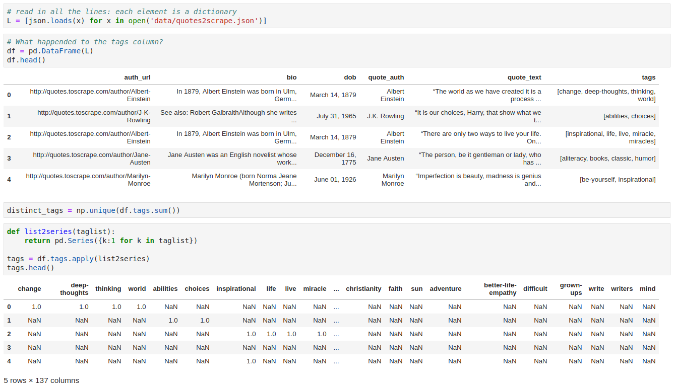
13. Text and features
1. Nominal feature encoding: One hot encoding
A column containing US states transforms into 50 feature columns
14. Features and models
1. Statistical Model: Inference
- A statistical model is a quantitative relationship between properties in observed data.
2. Prediction Model: Regression
- Regression Models attempt to predict the most likely quantitative value associated to an observation (feature).
3. Prediction Model: Classification
- Classification Models attempt to predict the most likely class associated to an observation (feature).
15. Modeling Pipeline
1. Transformer Classes(Transformer)
- Inputs and outputs are all numpy array
- Output data is also a numpy array
2. Sklearn Model Classes(Estimator)
Sklearn model classes (estimators) behave like transformers, but use outcomes (target variables) to fit and evaluate.
| Property | Example | Description |
|---|---|---|
| Initialize model parameters | lr = LinearRegression() | Create (empty) linear regression model |
| Fit the model to the data | lr.fit(data, outcomes) | Determines regression coefficients |
| Use model for prediction | lr.predict(newdata) | Use regression line make predictions |
| Evaluate the model | lr.score(data, outcomes) | Calculate the $R^2$ of the LR model |
| Access model attributes | lr.coef_ | Access the regression coefficients |
Note: Once fit, estimators are just transformers (predict <-> transform)
Design your own transformer():
class MyTrans(BaseEstimator, TransformerMixin):

    def __init__(self):

        pass

    def fit(self, X, y=None):

        return self

    def transform(self, X, y=None):

        return out
3. Building models with transformers and estimators
- Define your transformations; models.
- Transform input data to features.
- Use (transformed) features to fit model.
- Predict outcomes from features using fit model.
4. Pipeline
# Numeric columns and associated transformers
num_feat = ['total_bill', 'size']
num_transformer = Pipeline(steps=[
    ('scaler', pp.StandardScaler())
])

# Categorical columns and associated transformers
cat_feat = ['sex', 'smoker', 'day', 'time']
cat_transformer = Pipeline(steps=[
    ('intenc', pp.OrdinalEncoder()),
    ('onehot', pp.OneHotEncoder())
])

# preprocessing pipeline (put them together)
preproc = ColumnTransformer(transformers=[('num', num_transformer, num_feat), ('cat', cat_transformer, cat_feat)])

pl = Pipeline(steps=[('preprocessor', preproc), ('regressor', LinearRegression())])
16. Bias and Variance
Cross validation can reduce variance.
- Method 1: ```
scikit-learn k-fold cross-validation
from sklearn.model_selection import KFold
data sample
data = np.array([0.1, 0.2, 0.3, 0.4, 0.5, 0.6])
prepare cross validation
kfold = KFold(3, True, 1)
enumerate splits
for train, test in kfold.split(data): print(‘train: %s, test: %s’ % (data[train], data[test]))
train: [0.1 0.4 0.5 0.6], test: [0.2 0.3] train: [0.2 0.3 0.4 0.6], test: [0.1 0.5] train: [0.1 0.2 0.3 0.5], test: [0.4 0.6]
- Method 2
    `scores = cross_val_score(pipeline, X_train, y_train, cv=3)`

- Method 3
  **`GridSearchCV()`**
parameters = {
'max_depth': [2,3,4,5,7,10,13,15,18,None],
'min_samples_split':[2,3,5,7,10,15,20],
'min_samples_leaf':[2,3,5,7,10,15,20]
}
clf = GridSearchCV(DecisionTreeClassifier(), parameters, cv=5)
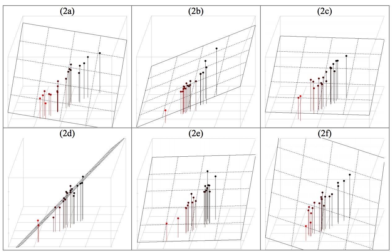
clf.fit(X_train, y_train) ``` ## 17. Examples ### 1. Regression with Multicollinearity * Linear regression with (perfectly) correlated features leads to high variance (unstable) models. * When the dataset ~1-dimensional in 3-dim space, fitting a plane is under-determined. * Use Principal Component Analysis to drop unneeded features.
18. Model Evaluation
1. Binary classification outcome
Accuracy treats TP the same as TN; not appropriate for class-imbalanced data(class imbalanced data is when the ratio of positive-negative outcomes is far from 1.)
When tackling class unbalanced condition, accuracy is not a good choice. We need the measurement to focus on more rare class.